NBER WORKING PAPER SERIES ADMINISTRATIVE DATA

NBER WORKING PAPER SERIES

ADMINISTRATIVE DATA LINKING AND STATISTICAL POWER PROBLEMS

IN RANDOMIZED EXPERIMENTS

Sarah Tahamont

Zubin Jelveh

Aaron Chalfin

Shi Yan

Benjamin Hansen

Working Paper 25657

http://www.nber.org/papers/w25657

NATIONAL BUREAU OF ECONOMIC RESEARCH

1050 Massachusetts Avenue

Cambridge, MA 02138

March 2019

We extend our sincere thanks to Melissa McNeill at the University of Chicago Crime Lab New

York for her work in developing the records matching algorithm employed in this paper. We

would also like to thank Leslie Kellam, Ryang Hui Kim, Srivatsa Kothapally, Jens Ludwig, Jim

Lynch, Mike Mueller-Smith, Aurelie Ouss, Greg Ridgeway, Jesse Rothstein and Greg Stoddard

for helpful comments on this project. We thank the Laura and John Arnold Foundation for its

generous support of the University of Chicago Crime Lab New York. Points of view or opinions

contained within this document are those of the author. They do not necessarily represent those of

the Laura and John Arnold Foundation or the National Bureau of Economic Research. Of course,

all remaining errors are our own. Corresponding Author: Sarah Tahamont, Email:

[email protected]

NBER working papers are circulated for discussion and comment purposes. They have not been

peer-reviewed or been subject to the review by the NBER Board of Directors that accompanies

official NBER publications.

rights reserved. Short sections of text, not to exceed two paragraphs, may be quoted without

explicit permission provided that full credit, including © notice, is given to the source.

Administrative Data Linking and Statistical Power Problems in Randomized Experiments

Sarah Tahamont, Zubin Jelveh, Aaron Chalfin, Shi Yan, and Benjamin Hansen

NBER Working Paper No. 25657

March 2019

JEL No. C1,C12,K42

ABSTRACT

The increasing availability of administrative data has led to a particularly exciting innovation in

public policy research, that of the “low-cost” randomized trial in which administrative data are

used to measure outcomes in lieu of costly primary data collection. Linking data from an

experimental intervention to administrative records that track outcomes of interest typically

requires matching datasets without a common unique identifier. In order to minimize mistaken

linkages, researchers will often use “exact matching” (retaining an individual only if all their

demographic variables match exactly in two or more datasets) in order to ensure that speculative

matches do not lead to errors in an analytic dataset. We argue that when this approach is used to

detect the presence of a binary outcome, this seemingly conservative approach leads to attenuated

estimates of treatment effects, and critically, to underpowered experiments. For marginally

powered studies, which are common in empirical social science, exact matching is particularly

problematic. In this paper, we derive an analytic result for the consequences of linking errors on

statistical power and show how the problem varies across different combinations of relevant

inputs, including the matching error rate, the outcome density and the sample size. We conclude

on an optimistic note by showing that machine learning-based probabilistic matching algorithms

allow researchers to recover a considerable share of the statistical power that is lost to errors in

data linking.

Sarah Tahamont

University at Albany,SUNY

[email protected]

Zubin Jelveh

University of Chicago

[email protected]

Aaron Chalfin

University of Pennsylvania

[email protected]

Shi Yan

Arizona State University

[email protected]

Benjamin Hansen

Department of Economics

1285 University of Oregon

Eugene, OR 97403

and NBER

[email protected]

1 Introduction

Among the more exciting developments in social science research is the innovation of the

increasingly ubiquitous “low-cost” randomized trial in which observations from an experi-

mental intervention are matched to administrative data in order to minimize primary data

collection and keep the costs of experimentation low. By linking together administrative

datasets, researchers can leverage the richness of information in pre-existing administrative

data sets and test the eﬀect of an intervention of interest on a host of outcomes in domains

as diverse as criminal justice, education and health (Kinner et al., 2013; Mueller-Smith,

2016; Petrou and Gray, 2011). Scholars are lauded for compiling and combining data from

multiple sources but, despite considerable attention to issues attendant to linking data in

the statistical literature (Fellegi and Sunter, 1969; Lahiri and Larsen, 2005; Neter et al.,

1965; Newcombe et al., 1959; Scheuren and Winkler, 1993, 1997), in practice, there is typ-

ically little discussion of how data sources are actually linked together in applied research.

It is not uncommon for researchers to have little information on the linking process itself,

because it is often the case that administrative agencies to do the linking in order to main-

tain conﬁdentiality. As a result, the description of the linking process that most research

papers provide is often limited to a footnote — if that.

When a unique identiﬁer is available in all of the datasets that require linking and

data quality is high, linking can, in some cases, be fairly trivial. These types of cross-

system unique identiﬁers are frequently available in Scandinavian countries (e.g. Black

et al., 2005; Dahl et al., 2014; Kuhn et al., 2011, among others). Unique identiﬁers in

the United States are essentially restricted to particular administrative system, requiring

linking across datasets which is typically both costly and results in some level of error. It

is often the case that unique identiﬁers are system-speciﬁc and virtually unknown outside

of the data (e.g. patient identiﬁers in hospital data or ﬁngerprint numbers in arrest data).

Even system-speciﬁc administrative identiﬁers that are known outside a database (e.g.

social security number or student identiﬁcation number) are not as reliable for linking

datasets as we might wish them to be because of problems with recording and reporting.

As a consequence, eﬀorts to link data from an experimental intervention to administrative

records that track outcomes of interest often require linking datasets that were not built

For an exception, see Khwaja and Mian (2005) an example from the applied economics literature,

which details the process for linking data and observes that matching errors will lead to attenuation in the

coeﬃcient estimates.

to be matched to one another and, which, often, lack a common unique identiﬁer. In the

absence of this identiﬁer, demographic characteristics like name and date of birth are used

to match data sets and, as a consequence, errors in data linkage are inevitable.

Matching errors can take on many forms depending on the record linkage problem

at hand. In this paper, we identify a special case of record linkage that is very common

but, unfortunately, is particularly diﬃcult to deal with: the case in which the goal is to

link datasets in an attempt to detect the presence of a binary outcome such as arrest or

high school graduation. Although the case we present is speciﬁc, our ﬁndings could extend

to a number of settings including program participation in Supplemental Nutritional As-

sistance Program (Courtemanche et al., 2018), employment prevalence measured through

unemployment insurance wage records (Mas and Johnston, forthcoming), injuries measured

through hospitalization data (Powell and Seabury, forthcoming), or ﬁnancial health mea-

sured through bankruptcy or liens (Dobkin et al., 2018).

At ﬁrst glance, it is not obvious why the form of the outcome variable should be a

ﬁrst order concern. To see why it is, we note that with a continuous outcome, when an

individual in an experimental sample cannot be linked to an outcome dataset, there is

a clear explanation of what has happened: the outcome data are missing. Consider, for

example, an outcome like a student’s score on a state standardized test. If Student A, a

participant in a study, is linked to a student record in a state’s education database, it is

possible that matching error might occur if the student was linked to the wrong student’s

outcome. But if, after the linking process, Student A’s record has not linked to a record in

the state database, then it is clear that the data are missing (either because of bad matching

or because the student did not take the exam).

. Ultimately, the primary question for the

researcher, in this case, is whether the data are missing at random or if statistical adjustment

is required to address the problem of non-random missing data. While this can be a thorny

problem in applied research, there is a litany of formal guidance and many associated “rules

of thumb” to help navigate this particular issue.

On the other hand, consider a diﬀerent scenario in which a researcher is interested in

evaluating whether a job training program for at-risk youth reduces the likelihood of arrest.

In constructing an analytic dataset, individuals whose names link to the post-intervention

arrest ﬁle are considered “arrested” and individuals whose names do not link to the arrest

Note that, in this case, there might even be an indicator for whether or not the student took the exam,

which might help diﬀerentiate between bad matching and missing data.

ﬁle are considered “not arrested.” Notably though, those individuals who cannot be found in

the arrest ﬁle did not necessarily have zero arrests — some of these individuals may not have

been found due to errors in their names, dates of birth, or other identifying characteristics

that were used to link the data. In this case, it is not clear what a non-linked record means:

does this mean that the individual has not been re-arrested or that the individual’s arrest

record cannot be found in the outcome dataset? Not limited to arrest, this issue is applicable

to any context in which the goal of the linking process is to determine the presence of an

outcome and there is no prior prediction for how many records should match — for example,

hospital utilization, college matriculation or program completion for an intervention.

There are two important features of our arrest scenario — or any scenario in which the

outcome of interest is binary — which bear further discussion. First, with a binary outcome

variable, the rate of successful record linking becomes the outcome density in the analytic

dataset. Because it is not clear a priori how many of the experimental records should link

to the outcome data, there is no way to use the match rate between datasets to evaluate the

quality of the match. Second, from a data-linking perspective, the most important thing

is to link the experimental observations to the correct outcome as opposed to linking to

the correct individual in the outcome data. That is, in this particular case, if Person A is

mistakenly linked to Person B in the outcome data, the mismatch will only be empirically

consequential if Person A and Person B have diﬀerent outcomes (e.g., Person A is arrested

and Person B is not arrested). This is not generally the case with a continuous outcome

where the outcome can take on many possible values.

These points distinguish this linking

case from other kinds of longitudinal record linking cases (Bailey et al., 2017; Feigenbaum,

2016) but, to our knowledge, this distinction has not been discussed in the prior literature

on administrative data matching.

A good match is critical, because bad matches introduce noise that obscures the re-

lationship between the outcome variable and the treatment variable. In the presence of

noisy matching, even a perfectly-executed randomized controlled trial will fail to deliver

an unbiased estimate of the eﬀectiveness of an intervention. In this paper, we show ana-

Consider that a low match rate in this context could either mean that there is a low re-arrest rate in

the sample or that there was a high rate of matching error.

It is important to note that this particular deﬁnition of matching error only applies when the experimen-

tal data is only being linked to the outcome data. If there are also additional variables in the administrative

data in addition to the outcome, those could generate problematic linking errors if they do not share the

demographic proﬁle of the experimental observation to which they are linked.

lytically that matching errors of this form will attenuate estimates of the treatment eﬀect

in an RCT. Critically though, while attenuation is an unwanted outcome, by far the most

insidious result of matching error is its eﬀect on ex-ante statistical power and, therefore,

on a researcher’s ability to detect a true treatment eﬀect when one exists (Type II errors).

While modest matching errors will lead to modest attenuation, given that few experiments

are overly well-powered, even small amounts of matching error can have outsize eﬀects on

Type II error rates. For rare outcomes (e.g. Gelber et al., 2016) and small sample sizes (e.g.

Fischbacher et al., 2001), both of which are common and even typical in randomized experi-

ments, matching errors are particularly problematic. For instance, medical studies, housing

lotteries, or educational experiments all are examples of potential experiments where some

of the most important outcomes are rare and could be measured with administrative data.

Researchers who conduct ex-ante power analyses, and subsequently link to administrative

data to detect the presence of their outcome of interest, will therefore overestimate their

power to detect eﬀects, often by a considerable margin. If null ﬁndings are less likely to be

published, attenuation bias can have dire consequences not only for individual papers but

also for entire literatures. Indeed, this form of publication bias (ﬁling papers in the “desk

drawer”) may contribute to the “replication crisis” in empirical social science (Camerer

et al., 2016; Gerber and Malhotra, 2008; Gilbert et al., 2016; Pashler and Wagenmakers,

2011; Vivalt, 2017).

How do researchers handle the problem of imperfect data linkage? Despite the existence

of a number of proposed linking methods (Lahiri and Larsen, 2005; Scheuren and Winkler,

1993, 1997), we observe that researchers, in practice, often use “exact matching”, consid-

ering an individual to be a match only if his or her demographic identiﬁers (i.e., name and

date of birth, etc.) match exactly in two or more datasets, in order to minimize incorrect

linkages in the data (Whitaker, 2004). Researchers impose stringent matching criteria in

order to ensure that speculative matches do not lead to errors in the dataset that will be

used to evaluate the intervention. This has been a popular approach to administrative data

linking (Gelber et al., 2016; Hser and Evans, 2008; Khwaja and Mian, 2005; Mueller-Smith,

2016), and is thought to be conservative, as it minimizes the probability that a bad match

will make it into the analytic dataset, thus keeping the data as “pure” as possible.

Concerns over the misuse of researcher degrees of freedom and speciﬁcation searching have likewise

spurred recommendations which include the use of very small α levels (Benjamin et al., 2018), which increases

the probability of Type II errors as a consequence of matching error even more.

A large literature considers the implications that measurement error can have for econometric models

This “conservative” approach to data linking is seemingly logical as it will minimize

false positive matches in which the wrong outcome data are linked to a given individual

in the study sample.

7,8

However, creating stringent character match requirements will,

by deﬁnition, increase false negative links. We argue that researchers should focus not

on “bad matches” but on the sum of false positive and false negative error rates in the

matching process. By allowing more false negatives in order to decrease false positive links,

“exact matching” can lead to a more matching error and more pronounced attenuation bias.

Instead, more ﬂexible matching strategies can reduce the rate of “missed” good matches

(even if they may slightly increase the rate of false positive links) and also decrease the

sum of the error rates. We further show that matches performed using machine-learning

algorithms (which draw on probabilistic matching techniques) can, in most cases, reduce

the sum of false positive and false negative error rates considerably by allowing for some

ﬂexibility in the match. Finally, we demonstrate how speciﬁcally minimizing the sum of

false positive and false negative error rates as the objective in a machine learning-based

matching algorithm leads to the lowest attenuation bias in regression estimates.

The paper proceeds as follows. First, we brieﬂy review the literature on matching errors

in empirical social science. Next, we derive an analytic result for the consequences of the

matching error on treatment eﬀect estimation and show that the sum of false positive and

false negative error rates is what matters, not either of these error rates in isolation. Next,

we present numerical estimates to demonstrate how the attenuation of treatment eﬀects and

the corresponding erosion of statistical power varies across diﬀerent combinations of relevant

inputs including the 1) the sum of false positive and false negative error rates, 2) the outcome

density, and 3) the sample size. Results suggest that, in most empirical applications, the

problem of bad data matching is not trivial — in a relatively large experiment (n = 750) with

a relatively non-dense outcome (

Y = 0.5), power would be 20% lower (0.6 instead of 0.8) in

the presence of a realistic amount of matching error. We proceed with an empirical example

but, to our knowledge, there is considerably less formal guidance with respect to how bad data matching

can confound randomized experiments. It is also worth noting that when scholars need to match datasets

without a common identiﬁer there is no “ground truth” to assess the quality of the match. Likewise, there is

often no prior about what the match rate should be, rendering it diﬃcult to diagnose whether the matching

procedure employed is suﬃcient or not.

We emphasize, again, that, in this case, that the “right” match in the special case that we discuss does

not depend on linking an observation to its own record, per se, but rather to a record with the same value

of the outcome.

It is important to note that the deﬁnition of matching error, as well as the implications for how matching

error will aﬀect coeﬃcient estimates varies by matching context. For example, Moore et al. (2014) show that

when estimating relative risk ratios, minimizing false positive links is the best approach to data linkage.

that shows the diﬀerence between conservative exact matching strategies and linking using

a simple machine learning algorithm, which incorporates probabilistic linking components.

We conclude on an optimistic note by showing that, in most cases, we can mitigate the

consequences of matching error using data linkages derived using a simple machine learning

algorithm.

2 Motivation and Context

Scholarly consideration of the implications of data linkage dates back to the early days of

computerized record linkage itself (Fellegi and Sunter, 1969; Neter et al., 1965; Newcombe

et al., 1959). However, despite multi-disciplinary recognition that linking errors have im-

plications for subsequent analyses (Aigner, 1973; Campbell, 2009; Khwaja and Mian, 2005;

Lahiri and Larsen, 2005; Neter et al., 1965; Scheuren and Winkler, 1993, 1997), it appears

that, until recently, by and large, scholars working with empirical applications have de-

voted relatively little attention to describing the techniques used to link data, evaluating

the quality of the matches in linked data, or to determining how their study conclusions

might have varied based on the use of diﬀerent data linking strategies.

In this section we provide a high-level conceptual overview of the essentials of data

linking in the social sciences. The purpose of this discussion is not to weigh in on best

practice in administrative data linking but instead to provide a framework to think about

how data linking can aﬀect downstream estimates of a treatment eﬀect of interest. In

this study, we use a very simple probabilistic matching algorithm in order to demonstrate

that even a basic implementation of probabilistic matching techniques can yield substantial

reductions in the bias introduced by linking errors and correspondingly large increases in ex

ante statistical power. Accordingly, we do not discuss the particulars of algorithm building

here but note, for interested readers, that excellent reviews can be found in Christen (2012)

and Winkler (2006).

Record linkage refers broadly to the practice of identifying records from diﬀerent datasets

that correspond to the same individual.

In some circumstances, linkages can be generated

For a notable exception, see the extensive work of Winkler and colleagues who have been tackling

related issues for decades with Census data (Scheuren and Winkler, 1993, 1997; Winkler, 2006).

For narrative clarity, we limit our discussion to the linkage of data containing records on persons. This

discussion would extend to groups or ﬁrms, but the characteristics available for linking might be diﬀerent.

using biometric indicators, such as ﬁngerprints, or other truly unique identiﬁers.

While

biometric data can lead to misidentiﬁcation in certain circumstances, linking using biomet-

ric indicators is generally considered more accurate than the traditional types of text-based

identiﬁers that we discuss in this paper (Watson et al., 2014) and may be suﬃciently ac-

curate to dramatically narrow the scope of matching errors and their resultant eﬀects on

empirical research. However, databases used to evaluate experimental interventions often do

not share a common unique identiﬁer, and even less often share common biometric identi-

ﬁers, so researchers have to rely on demographic information in order to identify individuals

in the data linkage process. Frequently-used demographic variables include an individual’s

name (including ﬁrst and last names, and sometimes a middle name or middle initial), date

of birth, social security number, gender, race, and ethnicity (for simplicity, hereinafter,

we refer to this set of information as a “demographic proﬁle”). When researchers use de-

mographic proﬁles to link individuals across datasets, the linking enterprise is necessarily

imperfect for a variety of reasons, including typographical errors, changes in names, geo-

graphic mobility and sometimes due to the intentional provision of inaccurate information

(e.g., an arrestee providing a false identify to a police oﬃcer).

Given that there is underlying uncertainty about the rate of errors in the data, re-

searchers need to develop a set of rules that govern whether two demographic proﬁles will

be treated as though they belong to the same observation. This process is inherently subjec-

tive and while there are long established models for data linkage (Fellegi and Sunter, 1969),

there has been little discussion about linking choices and processes in the applied literature

(Connelly et al., 2016; Goerge and Lee, 2001). We can organize approaches to data linkage

into several broad categories: manual review, deterministic linkage, probabilistic linkage

and hybrid linking approaches.

Borrowing techniques from archival matching of historical records, scholars with a small

number of cases to link can, and sometimes do, conduct a manual review of proﬁle dis-

agreements and decide whether or not two proﬁles should be considered to be a match.

Problems arise when there is limited information to work with and instead of being able to

For example, in the criminal justice domain, individuals are often tracked using unique ﬁngerprint-

based identiﬁers in criminal case processing data managed by multiple law enforcement agencies such as

police agencies, courts and prisons. For an application that uses this type of matching, (see Freudenberg

et al., 1998).

In this instance we deﬁne “manual review” as the comparison of two records by an individual as

compared to a computer, this is distinct from the kind of archival review referenced in Bailey et al. (2017)

during which trained reviewers use information from multiple sources to identify matches.

triangulate using contextual factors, the raters are simply guessing based on a ﬁxed set of

characteristics. In these cases, there is little reason to believe that manual review of cases

leads to higher accuracy when only demographic information is provided.

For example,

if two records share the same birthday, is Michael Smith a match for a record for Michael

Smyth, Mike Smith, or Mikey Smith? These might be typographical errors or nicknames,

but these might also be diﬀerent individuals. The scenario is further complicated when the

two records do not exactly share a birthday or an address. Likewise, studies in which the

pool of potential matches is large — for instance, a study of 200 students within a school

system with 50,000 students — it is impractical to conduct a thorough manual review, even

presuming that such a review could potentially produce more accurate matches.

When manual reviews are not possible, or even desirable, there are two approaches to

developing a set of rules that govern proﬁle linking (Mason and Tu, 2008; Winkler, 2006).

The ﬁrst, deterministic matching, refers to the practice of developing a set of criteria a

priori, and considering two demographic proﬁles to be the same individual if and only if

the original criteria are met. The strictest approach of this kind is “exact matching,” under

which a match is recognized only if all matching variables are identical across the two

proﬁles. Less stringent deterministic matching rules require only a subset of letters or digits

to match, such as the ﬁrst three or four letters of names, or the month and date digits of

dates of birth. Importantly, proﬁles only link when they meet all of the similarity criteria.

A second approach is probabilistic matching. Instead of making rules based on the num-

ber of agreeing letters and digits, probabilistic matching seeks to estimate the probability

that two proﬁles belong to the same individual.

Probabilistic linking typically leverages

techniques that can calculate the similarity of names based on phonetic computation (e.g.,

Soundex, Double Metaphone, etc.). The more reﬁned algorithms can also take into account

nicknames and the rarity of names in population (see for an example, Campbell et al., 2007).

A fully probabilistic linking approach was proposed by Lahiri and Larsen (2005) who advo-

cated using the matching weights in subsequent data analyses, re-weighting the data using

the matching probabilities, in order to account for the uncertainty in the linking process.

In fact, there is some reason to suspect that manual review of matches might lead to lower levels of

consistency due to reviewer fatigue, learning, or issues with inter-rater reliability.

According to our reading of the applied literature, “probabilistic matching” is used as a catch-all term

for any linkage method that incorporates a probabilistic technique, but, in practice, the term “probabilistic

matching” can refer to a number of diﬀerent approaches some of which are conceptually very diﬀerent from

one another.

Lahiri and Larsen (2005) builds on the work of Scheuren and Winkler (1993) who advocate for a similar

Carrying the matching probabilities into the analysis is the only pure form of probabilistic

data linking. However, in order to fully incorporate the probabilistic approach, a full set of

match weights is necessary. We were unable to ﬁnd an example of pure probabilistic linking

in the applied literature. This is perhaps because it is a computationally intensive strategy,

which may be intractable with large data sets.

In practice, the most common probabilistic data linking approach is actually a hybrid

method that combines probabilistic methods used to identify candidate links and then sets

a deterministic threshold to classify links, nonlinks (and, in some cases, potential links).

To our knowledge, references to probabilistic matching in the applied literature generally

include a deterministic component even if a linking threshold is not mentioned explicitly.

Although these approaches may be most accurately characterized as “hybrid probabilistic-

deterministic,” in order to be consistent with the bulk of the extant applied literature, we

will refer to probabilistic matching with a deterministic linking threshold as “probabilistic

matching” throughout the rest of the manuscript. Some researchers have used probabilistic

matching algorithms with deterministic thresholds, often in the form of commercial linking

packages (Gold et al., 2010; Heller, 2014; Kariminia et al., 2007). There are also studies

in which a third party, rather than the researchers, conducts the linking. In those cases,

the algorithm is determined by the linking agency and is often proprietary and therefore

unavailable to be interrogated by referees or other scholars in the ﬁeld (Binswanger et al.,

2007; Chowdry et al., 2013; Jiang et al., 2011; Zauber et al., 2012).

Diﬀerent approaches to matching can lead to considerable variation in match accuracy

based on how the approaches handle disagreements between proﬁles. There are two types

of matching errors: 1) false positives and 2) false negatives, and diﬀerent approaches to

matching will result in diﬀerent combinations of these matching errors since there is an

inherent trade-oﬀ between false positives and false negative matches (Christen and Goiser,

2007). To see why this will be the case, consider that raising the stringency of the criteria

that are used to identify a match will reduce the number of false positive matches at the

expense of increasing the number of false negative matches. On the other hand, less stringent

strategy, but with a blocked matrix of probabilities (as opposed to a fully deﬁned matrix of probabilities),

Lahiri and Larsen (2005) demonstrate that there are substantial gains to be made from fully deﬁning the

matrix of match probabilities. However, their method presumes that it is tractable to fully deﬁne this matrix,

which may not be feasible when linking large administrative databases.

The goal of the Fellegi and Sunter (1969) model is to minimize the number of ambiguous candidate

links that require additional review.

deterministic rules and hybrid probabilistic matching will result in a greater number of

false positive matches and fewer false negative matches (Zingmond et al., 2004). In general,

comparisons of matching algorithms have found that probabilistic matching algorithms have

higher overall accuracy rates than deterministic rules (Campbell, 2009; Campbell et al.,

2008; Gomatam et al., 2002; Tromp et al., 2011), or, at a minimum, have similar accuracy

rates to deterministic rules (Clark and Hahn, 1995).

Several studies have examined the eﬀects of matching errors on coeﬃcient estimates

when linking two separate ﬁles (Cryer et al., 2001; Lahiri and Larsen, 2005; Neter et al.,

1965; Scheuren and Winkler, 1993). At the inception of computerized data linkage, the

key conclusion from Neter and colleagues was that “the consequences of even small mis-

match rates can be considerable” (Neter et al., 1965, p. 1021). Moreover, researchers have

recognized that classiﬁcation errors, as a special case of classical measurement error, can

lead to downward bias in eﬀect size estimates (Aigner, 1973; Campbell, 2009; Khwaja and

Mian, 2005). For example, Khwaja and Mian (2005, p. 1379, emphasis original) cautioned

the readers that “when [their] algorithm matches a ﬁrm to a politician, but the match is

incorrect ... estimates of political corruption are likely to be underestimates of the true

eﬀect.”

While downward bias may not be a ﬁrst order concern when the biased estimates are

still statistically signiﬁcant, the bias can be very problematic when researchers are unable

to detect real relationships between an intervention and an outcome of interest, a problem

which may be greatly exacerbated by the diﬃculty of publishing ﬁndings that are not sta-

tistically signiﬁcant at conventional levels of conﬁdence. In the presence of publication bias,

statistical power problems generated by matching errors can have negative consequences

not only for individual papers but also, potentially, for entire literatures. We proceed by

deriving an analytic result that shows how matching errors attenuate coeﬃcient estimates

and how they aﬀect estimated standard errors. We then note the implications for statisti-

cal power empirically demonstrate that probabilistic matching can be extremely helpful in

most circumstances.

This result builds on Aigner (1973).

3 Derivation of Estimated Treatment Eﬀects, Standard Er-

rors and Statistical Power

In this section we derive the eﬀects of matching errors on the estimated treatment eﬀect,

ˆτ, as well as its standard error, se(ˆτ ), in a randomized experiment with a binary treatment

condition. We show that the eﬀects of matching errors on both quantities have a closed

form solution. The estimated ˆτ will be attenuated and the degree of attenuation will be

proportional to the sum of the false positive and false negative matching error rates. The

eﬀect of matching errors on se(ˆτ) is more complicated and may result in an increase or

decrease in the estimate of the standard error relative to the no matching error scenario. In

general, relative to the eﬀect on coeﬃcient estimates, standard errors are not very sensitive

to matching errors and, as a result, matching errors will always lead to a higher rate of

failing to reject a false null hypothesis, and in so doing, lead to a higher likelihood of

failing to detect a true treatment eﬀect of a randomized intervention under study. As we

show, matching errors can be very detrimental to statistical power in all but the largest

randomized experiments.

3.1 Estimated Treatment Eﬀect

We begin by showing that, in a randomized experiment, matching errors lead to attenuated

estimates of an average causal eﬀect in absolute terms. Consider a randomized control trial

with a study sample of n units of which a fraction, p, are assigned to treatment and the

remaining (1 − p) are assigned to a control condition. Information on this experimental

sample is stored in a dataset, E. We are interested in estimating the average treatment

eﬀect of our intervention on an outcome, y. In this case, the outcome measure is stored in

an administrative dataset, D, where the number of individuals in D is much larger than n.

In order to estimate the average treatment eﬀect, we need to match our experimental sample

to the outcomes stored in administrative dataset. If a record in E links to a record in D

then observed y = 1 and otherwise observed y = 0. The realized outcome for an individual

in E is given by the potential outcomes corresponding to the treatment condition:

)







(0) if T

= 0,

(1) if T

= 1

(1)

As such, the average treatment eﬀect of the intervention, τ can be computed as:

τ = E[y

(1) − y

(0)] = P (y

= 1|T

= 1) − P (y

= 1|T

= 0) (2)

where T is a treatment indicator. The process of matching the experimental data to the

outcome data can lead to two types of errors:

• False positive link (F P ): An instance in which an individual i has the true outcome

∗

= 0, but was incorrectly linked to some other individual’s record in D with y

∗

= 1

where i 6= j, such that in this case, the observed value of y after the linking process

is equal to 1.

• False negative link (F N): An instance in which an individual i has the true outcome

∗

= 1, but was not linked to a record in D. In this case, the observed value after the

linking process is y = 0.

It is important to note that since we are trying to match observations in E to a given

outcome in D, matching errors are only driven by whether the correct outcome is observed,

and not that the link refers to the same person in both datasets. Speciﬁcally, this means

that it would not be considered an error with respect to measuring the outcome if a record

in E is linked to the wrong person in D, provided the linked record had the same outcome

value as the true match. When records are matched to erroneous outcomes this will lead to

the following biased estimate of τ:

ˆτ = P (y

= 1|T

= 1) − P (y

= 1|T

= 0) (3)

To further characterize the nature of the bias in τ we introduce the following four deﬁnitions:

• True Positive Rate (T P R): P (y

= 1|y

∗

= 1), or the probability that an individual

with outcome y = 1 will be linked to an individual in D yielding an observed outcome

∗

= y = 1.

• True Negative Rate (T N R): P (y

= 0|y

∗

= 0), or the probability that an individual

with outcome y = 0 will not be linked to an individual in D yielding an observed

outcome y

∗

= y = 0.

• False Negative Rate (F N R): P (y

= 0|y

∗

= 1), or the probability that an individual

with outcome y

∗

= 1 will not be linked to an individual in D, yielding an observed

outcome y

∗

6= y. F N R is equivalent to 1 - T P R.

• False Positive Rate (F P R): P (y

= 1|y

∗

= 0), or the probability that an individual

with outcome y

∗

= 0 will be incorrectly linked to an individual in D, resulting in an

observed outcome y

∗

6= y. F P R is equivalent to 1 - T N R.

Then the observed, and potentially biased, treatment eﬀect can be written as:

ˆτ = P (y

= 1|T

= 1) − P (y

= 1|T

= 0)

j∈{0,1}

P (y

= 1, y

∗

= j|T

= 1) −

j∈{0,1}

P (y

= 1, y

∗

= j|T

= 0)

j∈{0,1}

P (y

= 1|y

∗

= j, T

= 1)P (y

∗

= j|T

= 1)

−

j∈{0,1}

P (y

= 1|y

∗

= j, T

= 0)P (y

∗

= j|T

= 0)

= T P R

P (y

∗

= 1|T

= 1) − T P R

P (y

∗

= 1|T

= 0)

+ F P R

P (y

∗

= 0|T

= 1) − F P R

P (y

∗

= 0|T

= 0) (4)

T P R

and T P R

are the true positive rates for the treatment and control groups, respec-

tively. Similarly, the false positive rate for the treatment and control groups are F P R

and F P R

. In the case where matching error rates are equivalent for both treatment

and control groups, as is expected under random assignment, we let T P R

= T P R

and

F P R

= F P R

. We can then re-write the expression more compactly:

ˆτ = T P R [P (y

∗

= 1|T

= 1) − P (y

∗

= 1|T

= 0)]

+ F P R [P (y

∗

= 0|T

= 1) − P (y

∗

= 0|T

= 0)] (5)

which can, in turn, be written as:

ˆτ = T P R [P (y

∗

= 1|T

= 1) − P (y

∗

= 1|T

= 0)]

− F P R [P (y

∗

= 1|T

= 1) − P (y

∗

= 1|T

= 0)] (6)

The bracketed term in (6) is simply τ, the true treatment eﬀect, which leads to the following

ﬁnal form in the case of equivalent matching error across treatment and control:

ˆτ = (T P R − F P R) τ (7)

We note that if the error rates were known, the true treatment eﬀect could be recaptured:

τ =

ˆτ

T P R − F P R

(8)

Non-zero matching error will always attenuate the absolute value of the true treatment

eﬀect.

Finally, we can re-write the denominator as 1 − (F NR + F P R) and generate two

critical insights. First, bias will be proportional to the total matching error rate. The ﬁnding

that the sum of false positive and false negative error rates drives the bias is particularly

important given the tendency toward “exact matching,” which is thought to minimize error,

but, in fact, reduces the number of false positive links while increasing the number of false

negative links. Second, under reasonable assumptions on the magnitude of the error rates

(i.e. when F N R + F P R < 1), ˆτ will be attenuated towards zero — that is, the estimated

treatment eﬀect will be too small.

3.2 Estimated Standard Errors

In Section 3.1 we showed that matching error leads to an attenuated estimate of the av-

erage treatment eﬀect and we further posited that bias introduced by matching errors will

reduce statistical power. However, in order to draw conclusions about the eﬀect of matching

errors on statistical power, we must also consider the eﬀect of matching error on estimated

standard errors. To see how matching error aﬀects σ

, note that the variance of τ is given

by:

p(1 − p)

(9)

where p is the proportion of the study sample enrolled in treatment, N is the sample size,

and σ

is the residual outcome variance from a regression of y on the treatment indicator, T .

Taking the square root of the quantity on the right-hand side of in (9) yields the estimated

standard error around τ .

The only remaining step is to estimate the residual variance. We note that in the case

of linear regression, σ

can be deﬁned via the residual sum of squares, and, with a binary

outcome and a binary treatment, results in the following form where y

and y

are the

If T P R = F P R then the previous equation is undeﬁned and the observed treatment eﬀect will equal

zero, but that situation is unlikely to occur in practice as it implies a random match.

number of individuals in the experimental group linked to records in the administrative

data for the treatment and control group, respectively (see derivation in Appendix B).

− ˆy

)

= y



1 −



+ y



1 −



(10)

While attenuation in the treatment eﬀect depends only on the the sum of false positive

and false negative error rates, matching error aﬀects the standard errors through the control

group mean, the treatment eﬀect, and the distribution of false positive and false negative

links. To see how the distribution of matching error types aﬀects the standard errors,

consider a scenario where there is no treatment eﬀect. When the false positive rate is

greater than the false negative rate, the number of instances where y = 1 will increase and

the outcome density will also increase. Conversely, when the false negative rate is higher

the number of instances where y = 0 will increase and the outcome density will decrease.

The outcome density that maximizes the variance is ¯y = 0.5.

Whether the standard

errors increase or decrease depends on the extent to which the errors move the outcome

density toward or away from 0.5. For example, if the overall mean is 0.4, but the matching

algorithm produces more false negatives than false positives, then the observed treatment

group mean will be less than 0.4 and the resulting standard error will shrink. The situation

is slightly more complicated when there is a treatment eﬀect, but we show in Appendix C

that Equation 10 is maximized when the control group mean plus the treatment eﬀect equal

0.5.

The interplay between these factors means that there will be scenarios in which matching

error will produce smaller standard errors when compared with the no error case. But in

the next section we show that even in these situations, matching error compromises a

researcher’s ability to detect a true treatment eﬀect.

3.3 Implications for Statistical Power

While attenuation of coeﬃcients can be troublesome, the eﬀect of matching errors on sta-

tistical power is a far greater concern. Due to resource constraints, few randomized experi-

ments are overpowered, so modest matching errors can have an outsize eﬀect on statistical

To see this, consider the scenario where there an equal number of individuals in the treatment and

control groups, then Equation 10 simpliﬁes to 2 y



1 −



. It is straightforward to show that this quantity

is maximized when y

power.

We begin by noting that since there is a closed form solution for the eﬀect of

matching errors on the estimated average treatment eﬀect and its standard error, there is

also a closed form solution for the eﬀect of matching errors on statistical power (1 − β). To

see this, consider that, for a given Type I error rate (α) and a standard error around the

average treatment eﬀect, the probability of a Type II error is given by:

β = Φ

− Φ

−1





−

(11)

where τ

is the hypothesized treatment eﬀect, σ

is the standard error, and Φ is the

cumulative distribution function for the normal distribution.

One minus this quantity is

statistical power. If the following condition holds, then power will always be lower under

matching error:

ˆτ

(12)

Since the true treatment eﬀect will be adjusted according to 1 − (F NR + F P R), Equation

12 can be re-written as:



1 − (F N R + F P R)



ˆτ



1 − (F N R + F P R)



As we discussed in the previous section, there will be situations in which σ

ˆτ

< σ

but in the Appendix we show that even in these situations the shrinkage in the standard

errors is never enough to oﬀset the consequences of coeﬃcient attenuation, and, therefore,

statistical power always decreases under matching error.

In the next section we show that even with modest matching errors, there can be large

declines in statistical power. Since, in the context of a randomized experiment, researchers

tend to set 1 − β on the basis of their relative tolerance for the risk of an underpowered

ﬁnding, the result is that researchers will undertake randomized experiments that are un-

derpowered relative to their desired power thresholds.

Ioannidis et al. (2017) show that the median statistical power for a large body of studies in economics,

most of them observational, is just 18%.

For smaller samples, Φ would be replaced by the cumulative distribution function for the t distribution.

4 Analytic Results

In order to provide a sense for the degree to which matching errors lead to attenuation in

experimental estimates, incorrect standard errors, and corresponding declines in statistical

power, we compute the Type II error rate over a range of reasonable parameter values.

We focus speciﬁcally on the outcome density for the control group ¯y

, the hypothesized

treatment eﬀect τ

, the sample size N and the matching error rates. Our goal here is to

demonstrate the dynamics of this problem and the contexts in applied research for which

it is likely to be especially pernicious.

4.1 Setup

In order to explore the eﬀect of matching errors under a range of diﬀerent parameterizations,

using the analytic results in Section 3, we derive closed form solutions for τ , se(τ) and,

ultimately, the Type II error rate, β, in two potential scenarios: one in which there are

no matching errors and another in which matching errors are present. While it is the

sum of false positive and false negative error rates (FPR+FNR) that dictates the degree of

attenuation in ˆτ, as we have shown, the extent to which matching errors aﬀect the standard

error around this estimate and, relatedly statistical power, will also depend on the ratio

of false positive to false negative match rates. We motivate our setup using a dichotomous

outcome, y and a binary treatment, T where, as before, p is the proportion of the sample

that is treated and the remaining 1 − p are untreated.

4.2 Main Results

Figure 1 contains four panels that report ex ante power calculations with and without

matching errors, corresponding to four control mean-eﬀect size combinations (¯y

∗

= 0.3,

0.5 and τ

= 15%, 25%) that are typical of power calculations in planning a randomized

experiment. In each panel, the total matching error rate — that is the sum of the false

negative and false positive match rates — is plotted on the X-axis while the Type II error

rate (β) is plotted on the Y -axis. The lines plot Type II error rates for a given sample size,

We begin our discussion with Panel (a) which corresponds with ¯y

∗

= 0.5 and τ = 25%,

The computational details of this exercise are described in the computational appendix to this paper.

the parameterization which is best powered for a given sample size. Consider, for example,

a very large experiment in which N = 2,000. In such an experiment, a Type II error will

be extraordinarily rare — approximately zero — in the absence of matching errors. Even

when the matching error rate is as high as 30%, the probability of a Type II error will

be approximately 3%, meaning that such an experiment will have a 97% probability of

detecting a treatment eﬀect of 25%. This is sensible as matching errors have little eﬀect on

statistical power when an experiment is extremely overpowered. However, due to resource

constraints, overpowered experiments are rare. A more realistic scenario is an experiment

in which N = 500. This sample size corresponds with the solid, red line in Panel (a). In

the absence of matching errors, this study has a Type II error rate of approximately 20%

which is considered by many researchers to be a reasonable default rule in conducting ex

ante statistical power calculations (Moher et al., 1994). Under even a relatively modest

matching error rate of 10%, Type II error rates rise to approximately 28%; with a 20%

matching error rate, the probability of a Type II error nearly doubles to 39%.

Another way to understand the impact of matching errors is to consider how much

larger the study would have to be to maintain a given Type II error rate, β. This too can

be seen in Figure 1. Referring to Panel (a), consider a study of size, N = 500 which has a

Type II error rate of approximately 20% in the absence of matching errors but a 38% Type

II error rate under 20% matching error. Here, it would take a 50% increase in the size of

the study (from N = 500 to 750) to return to the desired Type II error rate of 20%. As

resource constraints are often binding, increasing the size of a study by 50% is most often

infeasible.

The eﬀects of matching error on statistical power are even more dramatic with a less

dense outcome and a smaller treatment eﬀect of interest. In Panel (b), ¯y

∗

is ﬁxed at 0.5

but now we are interested in being able to detect a smaller treatment eﬀect, τ = 15%.

Now, even in the absence of matching error, we will need a larger sample size to detect a

treatment eﬀect of this magnitude (e.g. for N = 500, the Type II error rate at zero matching

error is greater than 60%). Focusing on the sample size (N = 1,500) that roughly yields

the default Type II error rate of 20% in the absence of matching errors. In this case, we see

that when the sum of false positive and false negative errors is at a reasonable level (15%)

Type II error rates will increase by approximately 50%, from 20% to around 30%. We see

a similar relationship when the treatment eﬀect of interest is 25% but the outcome is less

dense (Panel c). Finally, we turn to Panel (d) in which we have both a less dense outcome

¯y

∗

= 0.3 and a smaller treatment eﬀect of interest 15%. Here, even a very large experiment

will sometimes fail to detect a true treatment eﬀect as the Type II error rate for a study

of size N = 3,000 is approximately 25% in the absence of matching errors. In this case, a

reasonable matching error rate of 15%, takes the Type II error rate to 40%.

4.3 Extensions

Next, we consider two extensions of the simple model outlined in 4.1. Speciﬁcally, we allow

for the presence of a covariate that is correlated with the outcome and we consider the

implications of matching errors for tests of treatment heterogeneity.

4.3.1 Allowing for Covariates

The results reported in Section 4.2 presume that researchers do not have access to or,

at least, do not use pre-test covariates in estimating ˆτ . While a healthy debate exists

about the wisdom of controlling for covariates in a ﬁnite sample, it is common empirical

practice in analyzing randomized experiments to condition on covariates and estimate an

average treatment eﬀect by regressing y on both T and a vector of covariates, X (Angrist

and Pischke, 2009; Duﬂo et al., 2007). The wisdom behind controlling for covariates is

straightforward. Given that the treatment is randomized, X will be unrelated to T but

may be helpful in explaining y. The result is that residual variation will shrink and so too

will estimated standard errors. Thus, controlling for covariates will increase a researcher’s

power to detect treatment eﬀects and, in expectation, will not bias the estimated treatment

eﬀect. Given that the primary purpose of controlling for covariates in an experimental setup

is to increase statistical power, a natural question is whether doing so has implications for

the eﬀect of matching errors on statistical power.

In order to answer this question, we generate a covariate, X, that is correlated with y

∗

but which, by construction, is uncorrelated with T . For simplicity, we generate a dichoto-

mous X which is found in equal proportions in the treatment and control groups (though

all of the analytic results will also hold in the case in which X is continuous). The setup

is the same as before with the exception that we specify an imbalance parameter, r, which

governs the strength of the relationship between y

∗

and X. Speciﬁcally, r is diﬀerence in

the proportion of the sample for which y

∗

= 1 when X = 0 and when X = 1. In other

words, r represents the amount of imbalance in the outcome density between individuals

who possess characteristic X and those who do not. For example, if ¯y

∗

is 0.5, when r = 0.1,

¯y

∗

= 0.4 for the X = 1 group and 0.6 for X = 0 group, or vice versa. When r is large, y

∗

and X will be highly correlated and standard errors shrink by a relatively large amount.

In the demonstration below, we ﬁx r =0.1. However, the choice of r does not have a ﬁrst

order eﬀect on the extent to which matching errors lead to Type II errors.

We present

ﬁndings in Figure 2 in which Panels (a)-(d) correspond with the same parameterizations

shown in Figure 1. Referring to Panel (a) in which ¯y

∗

= 0.5 and τ = 25%, we see that,

compared to Figure 1, the y-intercept has shifted downwards reducing the probability of

Type II error when a covariate is added to the model. Without matching error, a sample of

N = 500 yielded a Type II error rate of approximately 20% in the absence of a covariate,

conditioning on a reasonably predictive covariate reduces the Type II error rate to just over

15%. In the case of this marginally powered sample (N = 500), a reasonable error rate of

15% doubles the Type II error. Referring to Panel (b) where the researcher would like to

detect a treatment eﬀect of 15%, we see that the consequences of matching errors continue

to be severe in the presence of a covariate with Type II error rates typically increasing

by between 50% and 75% with a relatively modest matching error rate of 15%. The key

takeaway is that despite the statistical power gains from covariate adjustment, matching

error remains a concern for experiments with marginally palatable Type II error rates.

4.3.2 Treatment Heterogeneity

A ﬁnal issue which is worth discussing concerns the task of testing for treatment het-

erogeneity in an experiment. Naturally tests for treatment heterogeneity will always be

underpowered relative to tests for the average treatment eﬀect. How though will these tests

be aﬀected by the presence of matching errors? We extend the setup in (4.3.1) and consider

a researcher who is interested in testing whether the eﬀect of treatment diﬀers according

to a dichotomous covariate, G which, to be concrete, we will assume is gender. In order to

The parameter r captures the strength of the relationship between X and y

∗

. Therefore, as r increases in

magnitude, statistical power increases, both in the absence and the presence of matching errors. However, the

relative gain statistical power is slightly larger when we do not condition on X. Across the parameterizations

we examine, in the absence of a covariate, the average loss of power under matching errors is 8.4%. When r

= 0.1, the loss of power is 8.8% when X is conditioned on. When r = 0.3, the average loss of power under

matching errors is 11.9% when X is conditioned on. Hence while a larger r is uniformly power enhancing, it

does mean that controlling for a covariate will be slightly less helpful in maximizing statistical power than

it otherwise would be.

determine whether the eﬀect of treatment is diﬀerent for men and women, the researcher

will specify the following regression model:

= α + τ T

+ πG

+ ρT

+ ε

(13)

Letting G = 1 denote the male group, in this model the treatment eﬀect for men will be

τ + ρ and the treatment eﬀect for women will be simply τ. Hence ρ represents the diﬀerence

in treatment eﬀects between men and women.

In the presence of matching errors, when estimating (13), τ will be incorrectly estimated.

However, the extent to which matching errors aﬀect the estimate of ρ depends on whether

the matching errors are orthogonal to G. In the case in which men and women are equally

likely to be incorrectly linked, the estimate of ρ will be unbiased; the estimate of the average

treatment eﬀect for men and women will be attenuated by an equal amount. However, if

the groups have diﬀerent error rates in the match, then the estimate of ρ will be biased.

This is likely to be a common problem. In the case of men and women, a number of papers

indicate that link rates are expected to be lower for women than for men because women

often change their names upon getting married (Bohensky et al., 2010; Maizlish and Herrera,

2005). The capacity to estimate heterogeneous treatment eﬀects is called into question if

match rates diﬀer by the category in question.

In the event that matching errors vary by group, the estimate of ρ will be biased upward

in the case that the G=1 group has more matching errors and will be biased downward

when the G=0 group has more matching errors. Thus, while matching errors are guaranteed

to lead to an attenuated estimate of the overall average treatment eﬀect, when the matching

errors vary by group, the direction of the bias in tests for treatment heterogeneity will be

ambiguous and will depend on the group speciﬁc matching error rates.

5 Empirical Example

Having established that matching errors can lead to a considerable number of Type II errors

in empirical applications, we next consider how to mitigate this problem. In Section 3, we

established that it is the sum of false positive and false negative error rates (rather than

either the false positive or false negative match rates individually) that controls the degree of

attenuation of parameter estimates and therefore, statistical power. While “exact matching”

will reduce the number of false positive links, it will, in general, not minimize the sum of

false positive and false negative error rates since the number of false negative links grows

because of the stringency of the matching criteria. There is, therefore, promise in testing

the performance of more ﬂexible matching strategies as an alternative to exact matching.

In this section, we show how a machine learning approach for probabilistic matching

can reduce the likelihood of Type II errors. There are two primary reasons to augment

traditional probabilistic matching techniques with machine learning methods. First, we deal

with a large dataset of over one million records. Probabilistic techniques involve computing

similarity metrics across a number of identifying characteristics such as name and date of

birth. It becomes prohibitively, computationally expensive to perform these calculations

for each potential record pair as the dataset size grows. Ideally, we would only perform

these computations for records for which we had some prior belief referred to the same

person. Techniques such as approximate nearest neighbors allow for fast detection of likely

matches that drastically reduce the number of comparisons that need to be made in the

linking process.

Second, the adaptivity of machine learning models for learning non-

linear functions and the practice of assessing performance on out-of-sample data lead to

predictive accuracy that outperforms linear models such as logistic regression. While not

limited to machine learning approaches, we augment our algorithm below by explicitly

having it minimize the right objective function for reducing the attenuation bias. The end

result is that we can trade oﬀ false positive and false negative matches to minimize the

attenuation due to matching error.

In order to explore the potential gains from probabilistic matching with machine learn-

ing, we need an empirical example. The reason for this is that while we can solve for the

bias that accrues from a given error rate, sample size and eﬀect size, the extent to which we

can reduce bias via a given matching strategy requires empirical data — names, dates of

birth and addresses, etc. which can be used to generate candidate matches. With empirical

data and a simulated randomized experiment in which a ground truth treatment eﬀect is

known, we can compare bias under exact matching and probabilistic matching with ma-

chine learning. We can therefore assess the extent to which probabilistic matching reduces

bias relative to exact matching for a given sample size and eﬀect size.

Although, Lahiri and Larsen (2005) show that a fully saturated matrix of comparisons yields the most

accurate probabilistic matching result, it has become increasingly common to observe matching cases that

render an unblocked linking procedure intractable.

We pause here to describe what the ideal empirical application will look like, noting that

the perfect application is not easily found. We will need two datasets: an “input” dataset

which contains information on a universe of research subjects including their treatment

indicators (our experimental dataset, E) and an “outcome” dataset with the universe of

candidate matches and their outcomes (our administrative dataset, D). The ideal appli-

cation must contain individually identiﬁed data that can be used to generate candidate

matches and should contain a “ground truth” identiﬁer that allows us to estimate a ground

truth treatment eﬀect in the absence of matching errors. We have identiﬁed empirical data

on individuals from the State of Oregon that meet each of these criteria (Hansen and Wad-

dell, 2018). We use the data to assign a placebo treatment indicator in order to simulate a

randomized experiment. Since we have a ground truth unique identiﬁer and a known data

generating process, we can understand the consequences of using either exact matching or

probabilistic matching on our estimates.

5.1 Empirical Simulation

For this study we use identiﬁed administrative records on 3 million charges ﬁled in Oregon

courts during the 1990-2012 window, maintained in the Oregon Judicial Information Net-

work (OJIN). These data have been used previously to show how legal access to alcohol

aﬀects criminality. Hansen and Waddell (2018) measured recidivism by recording whether

individuals appeared in dataset multiple times using exact matching. The individual records

in the OJIN data contain the following relevant variables: name, date of birth, race, incident

date, and a unique identiﬁcation number that links the same individuals across rows in the

dataset.

In order to simulate the linking scenario described above, we ﬁrst randomly sample 80%

of the data as input training data for our matching algorithm. These data represent our

administrative dataset, which we refer to as D. The remaining records are split equally

between a sample of records which we will use to optimize our matching algorithm, referred

to as E

, and a holdout sample from which we will derive our error rates for the algorithm,

. While D is at the record level, meaning a person can appear multiple times, we convert

There are situations where the two rows in the dataset will match on all relevant variables save for the

unique identiﬁer. As it is ambiguous whether these rows refer to diﬀerent individuals or if there is an error

in the unique identiﬁer, we drop these records from the empirical simulation. This reduces the number of

records to about one million.

both E

and E

to be at the person level by dropping duplicate rows with the same unique

identiﬁer. Our algorithm works by identifying instances in the training data where two

records are known to either refer to, or not refer to, the same person. We then compute

similarity measures a between these known pairs for the following ﬁelds: ﬁrst name, last

name, date of birth, race, and indictment date. A random forest model Breiman (2001)

run on these data produces probabilities for whether two records refer to the same person.

Further details of the algorithm appear in Jelveh and McNeill (2018). We use a cutoﬀ

threshold p

and we consider record pairs with predicted probabilities above p

to be links.

Recall that our objective is to minimize the quantity 1 − (F P R + F N R) and that it

is computed at the individual level, not the record level. Additionally, our measure of false

positives is a function of whether a link was made to the administrative data, not that

correct links are made at the individual level. Therefore, with E

we simulate the scenario

we have described in this paper. To do so, for each person in E

, we generate probabilities

for whether they are linked to individuals in D. We then estimate our objective for a range

of values for p

and choose the one that minimizes 1 − (F P R + F N R). To estimate out-

of-sample error rates, we then predict links between E

and D using the optimal p

and

report false positive and false negatives rates.

Table 1 compares the performance of the machine learning algorithm against exact

matching by name and date of birth when linking E

to D. As expected, the true positive

rate for exact matching is lower than that achieved by probabilistic matching. On the

other hand, exact matching is signiﬁcantly more likely to introduce false negatives. Most

importantly, as Table 1 shows, we substantially reduce sum of false positive and false

negative error rates by using a machine-learning strategy.

5.2 Empirical Simulation Results

To simulate matching error bias we follow the same procedure as in Section 4, this time

using actual linkage rates from exact and machine learning matching of our empirical data.

We explore the comparative performance of exact matching versus probabilistic matching

in Figure 3 which plots, for a given ¯y

∗

, τ and n combination, the share of linking errors

in the empirical data that are abated by using probabilistic matching as opposed to exact

matching. For example, referring to the ﬁgure, when ¯y

∗

= 0.5, τ = 15% and n = 500,

nearly 60 percent of linking errors that exist under exact matching are overturned when

we deploy a probabilistic matching algorithm. Across all parameterizations, probabilistic

matching with machine learning typically overturns half of the errors that exist under

exact matching. While our example here is limited to the performance of one probabilistic

algorithm, given our analytic results, we expect that the gains from using probabilistic

matching techniques will by and large outperform the stringency of “exact matching.”

6 Conclusion

We have shown that matching errors, even when introduced at random, have consequences

for our evidence base in empirical social science — in particular, by creating potentially

enormous challenges for developing evidence from randomized experiments, which remain

the gold standard for generating causal inferences about the social world. Our reading of

the prior literature is that scholars sometimes favor stringent matching criteria (i.e., exact

matching) in an eﬀort to minimize false positive matches with the goal of generating an

analytic dataset with as few errors as possible. However, a key insight from this research is

that the the sum of false positive and false negative error rates is the parameter that drives

the attenuation bias from matching errors, which means that stringent matching criteria

will increase, rather than minimize matching error bias. This is because while stringent

criteria minimize false positive matches, they substantially increase false negative matches.

As matching error aﬀects coeﬃcient estimates, there are descriptive as well as inferential

consequences.

In the presence of matching errors, for any sample size, coeﬃcients will be underesti-

mated, with degree of attenuation being proportional to the error rate in the match.

While

attenuation is unwelcome, matching errors have far more destructive consequences for sta-

tistical inference. This is because researchers who plan randomized experiments rarely have

more statistical power than they need to detect an eﬀect. The result is that a small degree

of attenuation can easily make an eﬀect size that was thought a priori to be detectable,

undetectable. As we show, this problem can be especially severe in experiments with small

samples or with larger samples and small eﬀect sizes. Taken study by study, this issue might

be dismissed as trivial, but because studies with “null results” are plausibly less likely to

be submitted and accepted for publication, as “low-cost randomized trials” gain traction,

It is worthwhile to note that the descriptive consequences of matching error cannot be resolved by

increasing sample size.

this problem stands to erode the quality of the social scientiﬁc evidence base — perhaps

substantially. While our analytical results apply speciﬁcally to randomized control trials,

similar patterns could also emerge for quasi-experimental settings. Likewise, although we

speciﬁcally focus on binary outcomes, continuous variables measuring outcomes like pro-

gram utilization, earnings, or duration could all suﬀer from similar problems when derived

from administrative data. In fact, it might even be more problematic if the lack of a match

is a recorded as a zero, a common mass point in those types of continuous variables.

On an optimistic note, we ﬁnd that probabilistic matching via machine learning algo-

rithms vastly outperforms exact matching and, in fact, in many scenarios approximates

a zero error scenario. We argue that these results provide compelling evidence that ex-

act matching should be abandoned in favor of probabilistic matching and that applied

researchers should pay greater attention to the way in which data linking is done more

generally.

Appendices

A Computational Details

In this appendix we provide additional details for how statistical power can be computed

under two possible states of the world: 1) in the absence of matching errors and 2) in

the presence of matching errors. We use the derivations in this appendix to empirically

demonstrate the eﬀect of matching errors on statistical power in a hypothetical experiment

in Section 5 of the paper.

We motivate the derivation by introducing a framework — a confusion matrix — that

governs the incidence of matching errors in a generic dataset. Each row of the confusion

matrix represents the incidence of an actual class while each column represents the instances

in a predicted class. The matrix thus allows an analyst to understand the extent to which

the algorithm is successful in classifying observations. In our context, we use a confusion

matrix to see how a matching algorithm has performed in correctly determining the presence

of an individual in a dataset.

In the following confusion matrix, y

∗

represents the true state of the world and y repre-

sents the observed state of the world after matching. The cells provide counts of the number

of true negatives, false negatives, false positives and true positives, respectively in linking

the data.

True state of the world

∗

= 0 y

∗

= 1

y = 0 T N F N

y = 1 F P T P

The diagonal entries of the matrix correspond to an alignment of the true and observed

states of the world — observations for which y

∗

= y = 0 are true negatives and observations

for which y

∗

= y = 1 are true positives. The oﬀ-diagonal entries provide us with the number

of matching errors. In particular, the 2,1 element of the matrix provides the number of false

positive matches — this is the number of times in which an observation which is truly y

∗

= 1 is mistakenly linked to y = 0.

Similarly, the 1,2 element of the matrix provides the

For consistency, we describe this as a mistaken link, when in practice, it is often the case that these

records would be non-links that are then assumed to have the value y = 0.

number of false negative matches where an observation that is truly y

∗

= 0 is mistakenly

linked to a record for which y = 1.

The table allows us to compute several quantities that are instrumental in deriving the

impact of matching errors on statistical power. We begin by noting that the matrix allows

us to compute four diﬀerent rates which allow us to measure the success of a given linking

strategy:

T P R =

T P

T P + F N

T NR =

T N

T N + F P

F P R = 1 − T N R

F NR = 1 − T P R

The true positive rate (T P R) is deﬁned as the number of linked positives divided by the

number of true positives (T P +F N). Likewise the true negative rate (T N R) is the number

of linked negatives divided by the number of true negatives (T N+F P ). The corresponding

false positive and false negative match rates are obtained by subtracting each of these

quantities from 1. As we show in Section 3 of the paper, estimated treatment eﬀects will

be attenuated under matching errors and the attenuation will be proportional to 1-F P R-

F NR. So long as F P R+F N R < 1, this will be strict attenuation towards zero but if

F P R+F NR exceeds 1 then there can be a change in the sign of the bias.

Overall, there are T P + F N actual failures and T P + F P observed failures. This

aspect of the table motivates our ﬁrst step in deriving a statistical power computation. In

particular, we can write down an expression for the number of failures in the control group

in the absence and presence of matching errors as follows:

∗

T =0

= (T P + F N) × (1 − p)

T =0

= (T P + F P ) × (1 − p)

∗

T =0

is the true number of failures in the control group and y

T =0

is the observed number

of failures where p is the proportion of the sample that receives the treatment.

Next, we consider how many successes there will be in the treatment group, with and

without matching errors. In order to compute these quantities we introduce a treatment

eﬀect, τ which, for simplicity, is expressed in percent (rather than percentage point) terms.

For our purposes, τ will be negative but this choice is trivial. The number of failures in the

treatment group will then be given by:

∗

T =1

= (T P + F N)(1 − τ ) × p

T =1

= (T P + F P )

1 − [τ (1 − F P R − F NR)]

× p

In the absence of matching errors, the number of observed failures will be equal to the

number of actual failures in the data multiplied by the proportion treated and one minus the

treatment eﬀect. When matching errors are present, the treatment eﬀect will be multiplied

by 1 − F P R − F N R to account for attenuation.

To appreciate how this works, consider a dataset of size N = 900, ﬁx P = 0.5 and

τ = 0.1 (10%) and use the following confusion matrix:

∗

= 0 y

∗

= 1

y = 0 T N =280 F N =100

y = 1 F P =20 T P =500

In this dataset, the FPR = 1 −

500

500+100

= 0.167 and the FNR = 1 −

280

280+20

= 0.067.

Accordingly, we will have the following numbers of failures in the treatment and control

groups in each of our two states of the world:

∗

T =0

= (T P + F N) × (1 − p) = 300

∗

T =1

= (T P + F N)(1 − τ ) × p = 270

T =0

= (T P + F P ) × (1 − p) = 260

T =1

= (T P + F P )

1 − [τ (1 − F P R − F NR)]

× p = 240

In the true state of the world, there are 300 failures in the control group and 270 in the

treatment group, reﬂecting the fact that τ = 0.1. With matching errors, the observed

number of failures in the control group is 260 and in the treatment group is 240. The

observed treatment eﬀect is smaller than 10%.

In order to compute statistical power to detect a given potential treatment eﬀect, we

need to compute a standard error which is computed according to:

var(ˆτ ) =

p(1 − p)

(14)

The square root of this quantity is the standard error around the estimated treatment eﬀect.

N and p are simply the sample size and the proportion treated but we will need to compute

which is the mean square error from a regression of either y

∗

or y on D, depending on

which state of the world we are in. We show how to compute σ

in absence and presence

of matching errors in Appendix B.

We can then compute statistical power according to:

β = Φ

−1



−

se(τ

)



Carrying through the numerical example from our confusion table, power to detect a treat-

ment eﬀect of 10% in these data are 90 percent in the true state of the world and just 67

percent in the state of the world with matching errors. What would have been an exceed-

ingly well-powered experiment is no longer well-powered in the presence of modest matching

errors.

B Deriving Outcome Variance

In this section we show how to compute the residual sum of squares with a binary outcome

and binary treatment in order to compute the σ

. Let ¯y

equal the control group mean and

τ the treatment eﬀect:

− ˆy

)

− ¯y

− τ T

)

We can decompose the above equation into four mutually exclusive groups determined

by whether an individual is in the treatment or control group, and whether their associated

outcome is y = 0 or y = 1.

i∈{i|y

=0,T

=0}

(−¯y

)

i∈{i|y

=1,T

=0}

(1 − ¯y

)

i∈{i|y

=0,T

=1}

(−¯y

− τ )

i∈{i|y

=1,T

=1}

(1 − ¯y

− τ )

= n

C,0

¯y

+ n

C,1

+ n

C,1

¯y

− n

C,1

2¯y

+ n

T,0

¯y

+ n

T,1

+ n

T,1

¯y

− n

T,1

2¯y

= n

¯y

+ n

C,1

− n

C,1

2¯y

+ n

¯y

+ n

T,1

− n

T,1

2¯y

= n

C,1

¯y

+ n

C,1

− n

C,1

2¯y

+ n

T,1

¯y

+ n

T,1

− n

T,1

2¯y

= n

C,1

(¯y

+ 1 − 2¯y

) + n

T,1

(¯y

+ 1 − 2¯y

)

= n

C,1

(1 − ¯y

) + n

T,1

(1 − ¯y

)

C Maximizing RSS

We now show why Equation 10 is maximized when the control group mean, ¯y

, plus the

treatment eﬀect, τ, equal 0.5. Let N

T,1

equal the number of individuals in the treatment

group with y = 1 and N

T,0

equal the number of individuals in the treatment group with

y = 0. Note that N

T,1

= (¯y

+ τ )N

and N

T,0

= N

(1 − (¯y

+ τ )).

− ˆy

)

− (¯y

+ τ T

))

For a given control group mean we will take derivatives with respect to τ , which means

we will only consider individuals in the treatment group. We can decompose the previous

equation into:

i∈T

− ˆy

)

= N

T,0

(−¯y

− τ )

+ N

T,1

(1 − ¯y

− τ )

= N

(1 − (¯y

+ τ ))(−¯y

− τ )

+ N

(¯y

+ τ )(1 − ¯y

− τ )

= N

(1 − ¯y

− τ )(¯y

+ τ )

+ N

(¯y

+ τ )(1 − ¯y

− τ )

= N

(1 − ¯y

− τ )(¯y

+ τ )(¯y

+ τ + 1 − α − τ)

= N

(1 − ¯y

− τ )(¯y

+ τ )

Let κ(τ ) = N

(1 − ¯y

− τ )(¯y

+ τ ), then taking derivatives with respect to τ :

dκ

dτ

= N

(−2¯y

− 2τ )

Setting the previous equation to zero and solving for τ leads to

¯y

+ τ = 0.5

D Proof for Power Attenuation

In this section we show that even when the standard error estimated under matching error

is smaller than the standard error estimated under no error, statistical power will still be

larger for the latter scenario. Let κ be True Positive Rate and ω be the False Positive Rate.

ˆτ

(κ − ω)τ

ˆτ

> (κ − ω)σ

ˆτ

− (κ − ω)σ

> 0

We can replace σ

ˆτ

and σ

with just the residual sum of squares components since all

other terms in their respective computations cancel out. Here N

∗

j,1

represents the number

of observations for which the true value of y, y

∗

= 1 and N

∗

j,0

represents the number of

observations for which the true value of y, y

∗

= 0. This allows us to write the last inequality

above as

j∈{T,C}

(κ N

∗

j,1

+ ω N

∗

j,0

)

1 −

κ N

∗

j,1

+ ω N

∗

j,0

∗

− (κ − ω)N

∗

j,1

1 −

∗

j,1

∗

> 0

j∈{T,C}

(κ N

∗

j,1

+ ω N

∗

j,0

)

(1 − κ)N

∗

j,1

+ (1 − ω)N

∗

j,0

∗

j,1

+ N

∗

j,0

− (κ − ω)

j,1

∗

j,0

∗

j,1

+ N

∗

j,0

> 0

j∈{T,C}

κ(1 − κ)N

∗2

j,1

+ ω(1 − ω)N

∗2

j,0

+ N

∗

j,1

∗

j,0

2ω(1 − κ) > 0

All terms in the last inequality are greater than zero, satisfying the condition.

References

Aigner, D. J. (1973). Regression with a binary independent variable subject to errors of

observation. Journal of Econometrics 1 (1), 49–59.

Angrist, J. D. and J.-S. Pischke (2009). Mostly harmless econometrics. Princeton, NJ:

Princeton University Press.

Bailey, M., C. Cole, M. Henderson, and C. Massey (2017, November). How well do auto-

mated methods perform in historical samples? Evidence from new ground truth. Working

Paper 24019, National Bureau of Economic Research.

Benjamin, D. J., J. O. Berger, M. Johannesson, B. A. Nosek, E. J. Wagenmakers, R. Berk,

K. A. Bollen, B. Brembs, L. Brown, C. Camerer, D. Cesarini, C. D. Chambers, M. Clyde,

T. D. Cook, P. De Boeck, Z. Dienes, A. Dreber, K. Easwaran, C. Eﬀerson, E. Fehr,

F. Fidler, A. P. Field, M. Forster, E. I. George, R. Gonzalez, S. Goodman, E. Green, D. P.

Green, A. G. Greenwald, J. D. Hadﬁeld, L. V. Hedges, L. Held, T. Hua Ho, H. Hoijtink,

D. J. Hruschka, K. Imai, G. Imbens, J. P. A. Ioannidis, M. Jeon, J. H. Jones, M. Kirchler,

D. Laibson, J. List, R. Little, A. Lupia, E. Machery, S. E. Maxwell, M. McCarthy, D. A.

Moore, S. L. Morgan, M. Munaf´o, S. Nakagawa, B. Nyhan, T. H. Parker, L. Pericchi,

M. Perugini, J. Rouder, J. Rousseau, V. Savalei, F. D. Sch¨onbrodt, T. Sellke, B. Sinclair,

D. Tingley, T. Van Zandt, S. Vazire, D. J. Watts, C. Winship, R. L. Wolpert, Y. Xie,

C. Young, J. Zinman, and V. E. Johnson (2018). Redeﬁne statistical signiﬁcance. Nature

Human Behaviour 2 (1), 6–10.

Binswanger, I. A., M. F. Stern, R. A. Deyo, P. J. Heagerty, A. Cheadle, J. G. Elmore, and

T. D. Koepsell (2007). Release from prison: A high risk of death for former inmates. The

New England Journal of Medicine 356 (2), 157–165.

Black, S. E., P. J. Devereux, and K. G. Salvanes (2005). Why the apple doesn’t fall far:

Understanding intergenerational transmission of human capital. American Economic

Review 95 (1), 437–449.

Bohensky, M. A., D. Jolley, V. Sundararajan, S. Evans, D. V. Pilcher, I. Scott, and C. A.

Brand (2010). Data linkage: a powerful research tool with potential problems. BMC

Health Services Research 10 (1), 346.

Breiman, L. (2001). Random forests. Machine Learning 45 (1), 5–32.

Camerer, C. F., A. Dreber, E. Forsell, T.-H. Ho, J. Huber, M. Johannesson, M. Kirchler,

J. Almenberg, A. Altmejd, T. Chan, E. Heikensten, F. Holzmeister, T. Imai, S. Isaksson,

G. Nave, T. Pfeiﬀer, M. Razen, and H. Wu (2016). Evaluating replicability of laboratory

experiments in economics. Science 351 (6280), 1433–1436.

Campbell, K. M. (2009). Impact of record-linkage methodology on performance indicators

and multivariate relationships. Journal of Substance Abuse Treatment 36 (1), 110–117.

Campbell, K. M., D. Deck, A. Cox, and C. Broederick (2007). The link king user manual:

Version v5.2.3.

Campbell, K. M., D. Deck, and A. Krupski (2008). Record linkage software in the public

domain: a comparison of link plus, the link king, and a ’basic’ deterministic algorithm.

Health Informatics Journal 14 (1), 5–15.

Chowdry, H., C. Crawford, L. Dearden, A. Goodman, and A. Vignoles (2013). Widening

participation in higher education: analysis using linked administrative data. Journal of

the Royal Statistical Society: Series A (Statistics in Society) 176 (2), 431–457.

Christen, P. (2012). Data matching: Concepts and techniques for record linkage, entity

resolution, and duplicate detection. New York, NY: Springer.

Christen, P. and K. Goiser (2007). Quality and complexity measures for data linkage and

deduplication. In F. J. Guillet and H. J. Hamilton (Eds.), Quality measures in data

mining, pp. 127–151. Berlin, Germany: Springer.

Clark, D. E. and D. R. Hahn (1995). Comparison of probabilistic and deterministic record

linkage in the development of a statewide trauma registry. Proceedings of the Annual

Symposium on Computer Application in Medical Care 1995, 397–401.

Connelly, R., C. J. Playford, V. Gayle, and C. Dibben (2016). The role of administrative

data in the big data revolution in social science research. Social Science Research 59,

1–12.

Courtemanche, C. J., A. Denteh, and R. Tchernis (2018). Estimating the associations be-

tween snap and food insecurity, obesity, and food purchases with imperfect administrative

measures of participation. Technical report, National Bureau of Economic Research.

Cryer, P. C., S. Westrup, A. C. Cook, V. Ashwell, P. Bridger, and C. Clarke (2001). Inves-

tigation of bias after data linkage of hospital admissions data to police road traﬃc crash

reports. Injury Prevention 7 (3), 234–241.

Dahl, G. B., A. R. Kostøl, and M. Mogstad (2014). Family welfare cultures. The Quarterly

Journal of Economics 129 (4), 1711–1752.

Dobkin, C., A. Finkelstein, R. Kluender, and M. J. Notowidigdo (2018). The economic

consequences of hospital admissions. American Economic Review 108 (2), 308–352.

Duﬂo, E., R. Glennerster, and M. Kremer (2007). Using randomization in development

economics research: A toolkit. In T. P. Schultz and J. A. Strauss (Eds.), Handbook of

development economics, Volume 4 of Handbook of Development Economics, pp. 3895–

3962. Amsterdam, the Netherlands: North-Holland.

Feigenbaum, J. J. (2016). Automated census record linking: A machine learning approach.

Working Paper.

Fellegi, I. P. and A. B. Sunter (1969). A theory for record linkage. Journal of the American

Statistical Association 64 (328), 1183–1210.

Fischbacher, U., S. G¨achter, and F. Ernst (2001). Are people conditionally cooperative?

evidence from a public goods experiment. Economics Letters 71 (3), 397–404.

Freudenberg, N., I. Wilets, M. B. Greene, and B. E. Richet (1998). Linking women in jail to

community services: Factors associated with rearrest and retention of drug-using women

following release from jail. Journal of the American Medical Women’s Association 53 (2),

89–93.

Gelber, A., A. Isen, and J. B. Kessler (2016). The eﬀects of youth employment: Evidence

from new york city lotteries. The Quarterly Journal of Economics 131 (1), 423–460.

Gerber, A. S. and N. Malhotra (2008). Do statistical reporting standards aﬀect what is

published? publication bias in two leading political science journals. Quarterly Journal

of Political Science 3 (3), 313–326.

Gilbert, D. T., G. King, S. Pettigrew, and T. D. Wilson (2016). Comment on “Estimating

the reproducibility of psychological science”. Science 351 (6277), 1037.

Goerge, R. M. and B. J. Lee (2001). Matching and cleaning administrative data. In

M. Ver Ploeg, R. A. Moﬃtt, and C. F. Citro (Eds.), Studies of welfare populations: Data

collection and research issues, pp. 197–219. Washington, DC: National Academy Press.

Gold, M., S. Dugdale, R. J. Woodman, and K. A. McCaul (2010). Use of the Australian

Childhood Immunisation Register for vaccine safety data linkage. Vaccine 28 (26), 4308–

4311.

Gomatam, S., R. Carter, M. Ariet, and G. Mitchell (2002). An empirical comparison of

record linkage procedures. Statistics in Medicine 21 (10), 1485–1496.

Hansen, B. and G. R. Waddell (2018). Legal access to alcohol and criminality. Journal of

Health Economics 57, 277–289.

Heller, S. B. (2014). Summer jobs reduce violence among disadvantaged youth. Sci-

ence 346 (6214), 1219–1223.

Hser, Y. I. and E. Evans (2008). Cross-system data linkage for treatment outcome eval-

uation: lessons learned from the california treatment outcome project. Evaluation and

Program Planning 31 (2), 125–135.

Ioannidis, J. P., T. D. Stanley, and H. Doucouliagos (2017). The power of bias in economics

research. The Economic Journal 127 (605), F236–F265.

Jelveh, Z. and M. McNeill (2018). Downstream impact of probabilistic matching quality

on prediction performance. In Progress.

Jiang, D., M. Walsh, and L. K. Augimeri (2011). The linkage between childhood bullying

behaviour and future oﬀending. Criminal Behaviour and Mental Health 21 (2), 128–135.

Kariminia, A., T. Butler, S. Corben, M. Levy, L. Grant, J. Kaldor, and M. Law (2007).

Extreme cause-speciﬁc mortality in a cohort of adult prisoners–1988 to 2002: A data-

linkage study. International Journal of Epidemiology 36 (2), 310–316.

Khwaja, A. I. and A. Mian (2005). Do lenders favor politically connected ﬁrms? rent

provision in an emerging ﬁnancial market. The Quarterly Journal of Economics 120(4),

1371–1411.

Kinner, S. A., S. Forsyth, and G. M. Williams (2013). Systematic review of record linkage

studies of mortality in ex-prisoners: why (good) methods matter. Addiction 108 (1),

38–49.

Kuhn, P., P. Kooreman, A. Soetevent, and A. Kapteyn (2011). The eﬀects of lottery prizes

on winners and their neighbors: Evidence from the Dutch postcode lottery. American

Economic Review 101 (5), 2226–2247.

Lahiri, P. and M. D. Larsen (2005). Regression analysis with linked data. Journal of the

American Statistical Association 100 (469), 222–230.

Maizlish, N. A. and L. Herrera (2005). A record linkage protocol for a diabetes registry at

ethnically diverse community health centers. Journal of the American Medical Informat-

ics Association 12 (3), 331–337.

Mas, A. and A. Johnston (forthcoming). Potential unemployment insurance duration and

labor supply: The individual and market-level response to a beneﬁt cut. Journal of

Political Economy.

Mason, C. A. and S. Tu (2008). Data linkage using probabilistic decision rules: a primer.

Birth Defects Research (Part A) 82 (11), 812–821.

Moher, D., C. S. Dulberg, and G. A. Wells (1994). Statistical power, sample size, and their

reporting in randomized controlled trials. JAMA 272 (2), 122–124.

Moore, C. L., J. Amin, H. F. Gidding, and M. G. Law (2014). A new method for assessing

how sensitivity and speciﬁcity of linkage studies aﬀects estimation. PloS ONE 9 (7),

e103690.

Mueller-Smith, M. (2016). The criminal and labor market impacts of incarceration. Working

paper.

Neter, J., E. S. Maynes, and R. Ramanathan (1965). The eﬀect of mismatching on the

measurement of response errors. Journal of the American Statistical Association 60 (312),

1005–1027.

Newcombe, H. B., J. M. Kennedy, S. Axford, and A. P. James (1959). Automatic linkage

of vital records. Science 330 (3381), 954–959.

Pashler, H. and E.-J. Wagenmakers (2011). Editors’ introduction to the special section on

replicability in psychological science: A crisis of conﬁdence? Perspectives on Psychological

Science 7 (6), 528–530.

Petrou, S. and A. Gray (2011). Economic evaluation alongside randomised controlled trials:

design, conduct, analysis, and reporting. BMJ 342, d1548.

Powell, D. and S. Seabury (forthcoming). Medical care spending and labor market outcomes:

Evidence from workers’ compensation reforms. American Economic Review.

Scheuren, F. and W. E. Winkler (1993). Regression analysis of data ﬁles that are computer

matched, part i. Survey Methodology 19 (1), 39–58.

Scheuren, F. and W. E. Winkler (1997). Regression analysis of data ﬁles that are computer

matched, part ii. Survey Methodology 23 (2), 157–165.

Tromp, M., A. C. Ravelli, G. J. Bonsel, A. Hasman, and J. B. Reitsma (2011). Results

from simulated data sets: probabilistic record linkage outperforms deterministic record

linkage. Journal of Clinical Epidemiology 64 (5), 565–572.

Vivalt, E. (2017). The trajectory of speciﬁcation searching and publication bias across

methods and disciplines. Working paper.

Watson, C. I., G. P. Fiumara, E. Tabassi, W. J. Salamon, and P. A. Flanagan (2014).

Fingerprint vendor technology evaluation. Report, NIST.

Whitaker, R. C. (2004). Predicting preschooler obesity at birth: The role of maternal

obesity in early pregnancy. Pediatrics 114 (1), e29–e36.

Winkler, W. E. (2006). Overview of record linkage and current research directions. Report,

U.S. Census Bureau.

Zauber, A. G., S. J. Winawer, M. J. O’Brien, I. Lansdorp-Vogelaar, M. van Ballegooijen,

B. F. Hankey, W. Shi, J. H. Bond, M. Schapiro, J. F. Panish, E. T. Stewart, and J. D.

Waye (2012). Colonoscopic polypectomy and long-term prevention of colorectal-cancer

deaths. The New England Journal of Medicine 366, 687–696.

Zingmond, D. S., Z. Ye, S. L. Ettner, and H. Liu (2004). Linking hospital discharge and

death records—accuracy and sources of bias. Journal of Clinical Epidemiology 57 (1),

21–29.

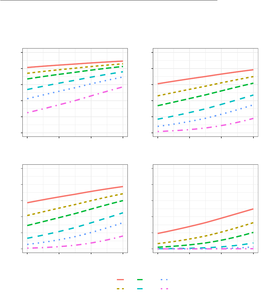
Figure 1: Matching Error and Type II Error Rates By Outcome Density and Treatment

Eﬀect Size

0.0

0.2

0.4

0.6

0.8

1.0

0 10 20 30

FPR + FNR

Type II Error

Control Mean = 30%, Effect Size = 15%

0.0

0.2

0.4

0.6

0.8

1.0

0 10 20 30

FPR + FNR

Type II Error

Control Mean = 50%, Effect Size = 15%

0.0

0.2

0.4

0.6

0.8

1.0

0 10 20 30

FPR + FNR

Type II Error

Control Mean = 30%, Effect Size= 25%

0.0

0.2

0.4

0.6

0.8

1.0

0 10 20 30

FPR + FNR

Type II Error

Control Mean = 50%, Effect Size= 25%

sample_size

500

750

1000

1500

2000

3000

Note: Figures plot the Type II error rate (β) as a function of the total matching error

rate for a given hypothesized eﬀect size and control mean. In each plot, Type II error rates

are plotted for sample sizes that range from N = 500 to N = 3,000.

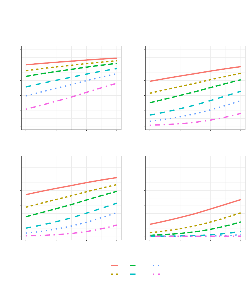
Figure 2: Matching Error and Type II Error Rates w/ Covariate Adjustment By Outcome

Density and Treatment Eﬀect Size

0.0

0.2

0.4

0.6

0.8

1.0

0 10 20 30

FPR + FNR

Type II Error

Control Mean = 30%, Effect Size = 15%

0.0

0.2

0.4

0.6

0.8

1.0

0 10 20 30

FPR + FNR

Type II Error

Control Mean = 50%, Effect Size = 15%

0.0

0.2

0.4

0.6

0.8

1.0

0 10 20 30

FPR + FNR

Type II Error

Control Mean = 30%, Effect Size= 25%

0.0

0.2

0.4

0.6

0.8

1.0

0 10 20 30

FPR + FNR

Type II Error

Control Mean = 50%, Effect Size= 25%

sample_size

500

750

1000

1500

2000

3000

Note: Figures plot the Type II error rate (β) as a function of the total matching error

rate for a given hypothesized eﬀect size, control mean, and correlated covariate. In each

plot, Type II error rates are plotted for sample sizes that range from N = 500 to N =

3,000.

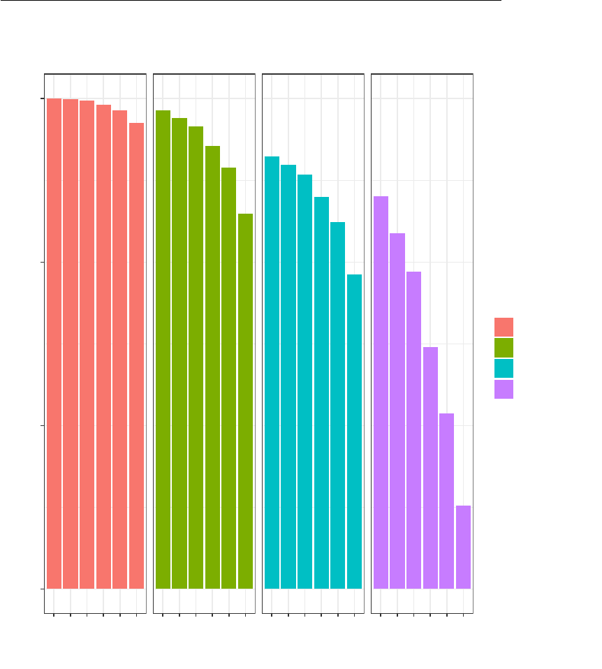
Figure 3: Percent of Exact Matching Errors Overturned

500

750

1000

1500

2000

3000

500

750

1000

1500

2000

3000

500

750

1000

1500

2000

3000

500

750

1000

1500

2000

3000

0.0

0.2

0.4

0.6

Sample Size

Share Fixed

Control Mean,

Treatment Effect

30, 15

30, 25

50, 15

50, 25

Note: Figures plot the share of errors under exact matching that are overturned when

a probabilistic matching algorithm is employed. Each panel represents a diﬀerent control

mean and treatment eﬀect combination.

Table 1: Performance metrics across matching schemes

Exact Matching Probabilistic Matching

False Negative Rate 14.0% 0.8%

False Positive Rate 0.0% 6.2%

F NR + F P R Rate 14.0% 7.0%

Note: Average error rates from empirical matches of OJIN data.